
First, a coffee
Stonkholders,
Imagine a café sells a coffee for €5.
In this example, one euro initially buys one dollar. Your coffee costs $5.
The euro then rises to $1.20. The café leaves its menu untouched. The same coffee now costs $6.
The coffee did not become more expensive in euros. The euro became more expensive in dollars.
Now replace the coffee with a token, and the euro with STONK.
Suppose one TOKEN trades for one STONK. STONK rises from $1 to $10, while that exchange rate remains unchanged.
One TOKEN is now worth $10 rather than $1.
It has appreciated tenfold in dollars without appreciating at all against STONK.
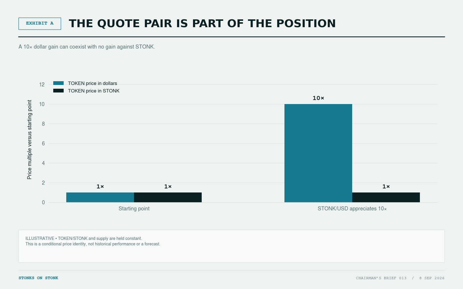
The important phrase is “while that exchange rate remains unchanged.” This is conditional arithmetic, not a forecast. Buyers and sellers can change how much STONK a TOKEN commands.
A 10× STONK move combined with a halving against STONK produces a 5× dollar result. A doubling against STONK produces a 20× result.
The arithmetic is multiplication:
TOKEN’s dollar price = STONK per TOKEN × dollars per STONK.
The dollar chart combines two prices. It does not tell us, by itself, which one moved.
Management has determined that the second ticker requires supervision.
The market cap is not the money in the machine
Think of a liquidity pool as a trading machine with two compartments: project tokens in one, the quote asset in the other.
A buyer puts quote tokens in and takes project tokens out. A seller does the reverse. An automated market maker, or AMM, supplies the pricing rule. In a conventional constant-product pool, buying more project tokens progressively makes the next token more expensive. SOURCE 01Uniswap — V2 pricingOpen source ↗
Consider a simplified market. There are 1,000 TOKEN in total. The pool holds 100 TOKEN and 100 STONK. One TOKEN trades for one STONK, and STONK is worth $1.
The pool is worth $200: $100 of TOKEN and $100 of STONK.
The token’s market capitalization is $1,000: the assumed 1,000-token supply multiplied by the $1 marginal price.
The liquidity ratio is therefore 20%.
Market capitalization is not the amount invested, and it is not what everyone could collectively withdraw at that price. Similarly, the $200 pool does not contain $200 of STONK. Half its marked value is the project’s own inventory.
For this Brief, liquidity ratio means pool value divided by a stated market-cap measure. Quote reserves means the quote tokens actually held. Executable depth means how much buying or selling can occur within a specified price movement.
Those are three different measurements.
Three ways to go up 10×
Start each scenario with the same $200 pool and $1,000 market cap. Use an ordinary real-reserve constant-product pool, fixed supply, no fees or taxes, and no liquidity added or removed.
| What moved? | STONK/USD | TOKEN/STONK | TOKEN/USD | Ending pool value | Pool / market cap |
|---|---|---|---|---|---|
| STONK alone | 10× | 1× | 10× | $2,000 | 20.0% |
| TOKEN alone | 1× | 10× | 10× | $632 | 6.3% |
| Both | 2× | 5× | 10× | $894 | 8.9% |
Calculated examples. Ending market cap is $10,000 in every row; dollar amounts are rounded. The calculations are reproduced in the technical appendix.
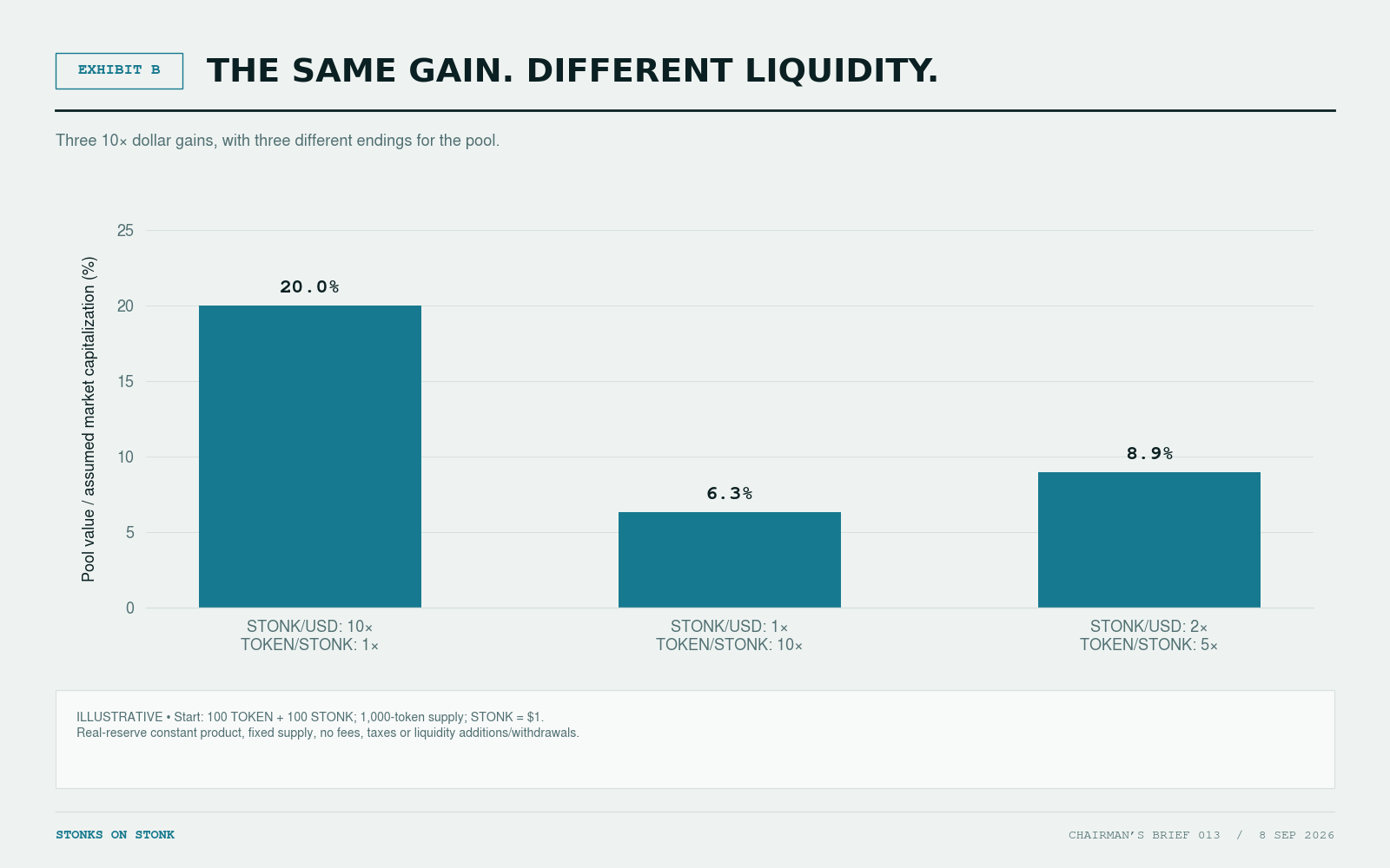
In the first case, neither compartment changes. Both simply become worth ten times as much in dollars. Market cap also increases tenfold. The ratio remains 20%.
In the second, TOKEN commands more STONK. The pool ends with approximately 31.62 TOKEN and 316.23 STONK. Its inventory has changed, and market cap has outrun its total value.
No liquidity withdrawal is required to explain the lower ratio.
The third combines both effects.
The quote-only result is not unique to constant product. With unchanged inventory, relative price and supply, pure quote-dollar repricing scales pool value and market cap together in a concentrated pool too. The reserve-rebalancing calculations are the part that depends on the AMM’s design.
The reverse also holds: if STONK halves while everything else stays fixed, dollar pool value and market cap both halve. An unchanged ratio does not mean an unchanged dollar position.
Why the same buy does not buy the same candle
Now give three hypothetical tokens the same $1 million market cap, but different pool sizes.
Spend $1,000 worth of the quote asset buying each one.
| Pool / market cap | Total pool value | Quote-side value | Average purchase-price premium | Final marginal-price increase |
|---|---|---|---|---|
| 5% | $50,000 | $25,000 | 4.00% | 8.16% |
| 10% | $100,000 | $50,000 | 2.00% | 4.04% |
| 20% | $200,000 | $100,000 | 1.00% | 2.01% |
Calculated fee-free constant-product examples. Quote/USD is fixed during the trade. No taxes, other trades, arbitrage or liquidity changes. These are not execution estimates for STONKS, DEX or KNOTS.
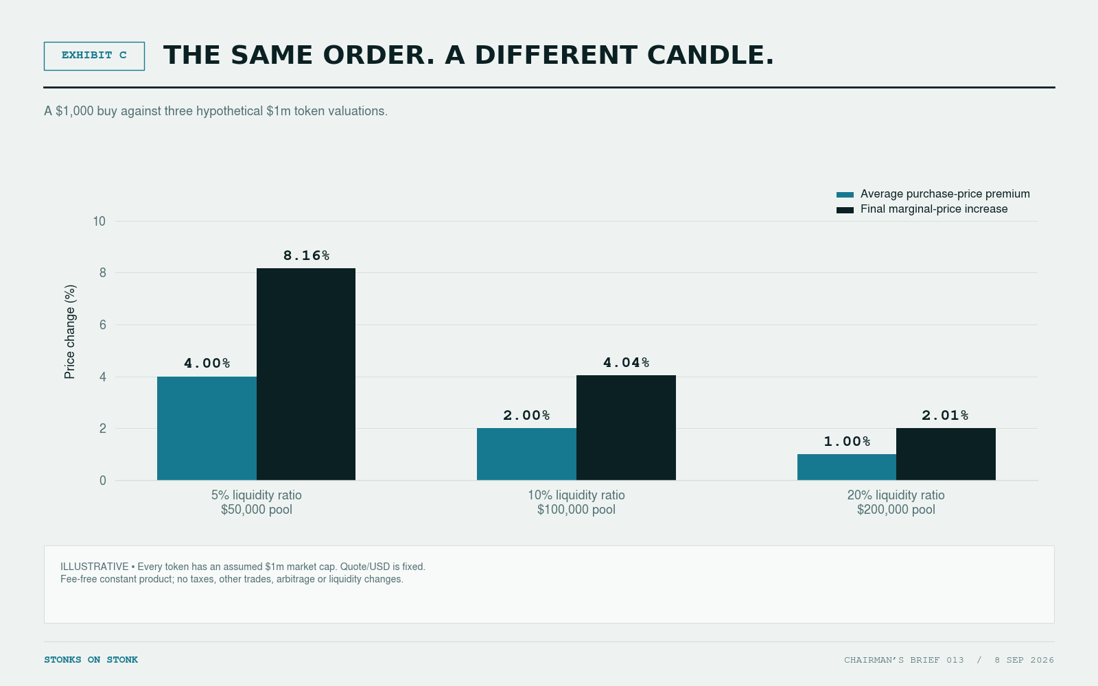
Same valuation. Same order. Different price movement.
The smallest pool produces approximately four times the percentage marginal-price movement of the largest because the order is larger relative to its reserves.
A larger candle does not necessarily mean a larger inflow.
The two right-hand columns answer different questions. In the first row, the buyer pays an average premium of 4%. The final pool price is 8.16% higher. The order did not execute entirely at that final price; it moved through progressively higher prices.
Neither measure should be confused with execution slippage: the difference between a quoted outcome and what actually arrives if conditions change before execution. Trading fees and token taxes are additional effects. SOURCE 02Raydium — Slippage and price impactOpen source ↗
Lower depth also makes selling more consequential. Exact buy and sell percentages need not be symmetric, especially when comparing different order-sizing conventions.
The governing question is trade size relative to usable liquidity, not the liquidity ratio in isolation.
A familiar example: buying on PumpSwap
The denominator does not have to be exotic.
Pump documents a native bonding-curve launch followed by migration to PumpSwap. Its current native quote options include SOL and USDC. Here we use a fictional SOL-quoted token already trading after graduation. SOURCE 03Pump — Bonding-curve overviewOpen source ↗SOURCE 04Pump — FeesOpen source ↗
Our hypothetical PumpSwap pool holds 50 million TOKEN and 500 SOL. SOL is worth $100. TOKEN therefore starts at 0.00001 SOL, or $0.001.
With an assumed one-billion-token supply, valuation is $1 million, pool value is $100,000 and the liquidity ratio is 10%. Using the full assumed supply is a valuation convention, not an independently verified circulating-market-cap calculation.
A $1,000 purchase adds 10 SOL. Under fee-free constant-product arithmetic, it receives approximately 980,392 TOKEN. The average purchase price is $0.0010200, while the final marginal price is $0.0010404: a 2% average premium and a 4.04% marginal-price increase. PumpSwap’s program documentation supplies the constant-product baseline; this illustration assumes no virtual quote adjustment. SOURCE 05Pump — PumpSwap program READMEOpen source ↗
The assumed valuation rises by $40,400 following a $1,000 order. That is the supply being marked at a new marginal price—not $40,400 arriving in the pool.
Now reset to the original inventory and let SOL double to $200, with TOKEN/SOL unchanged.
| Before each separate hypothetical buy | SOL at $100 | SOL at $200 |
|---|---|---|
| Token valuation | $1 million | $2 million |
| Pool value | $100,000 | $200,000 |
| Liquidity ratio | 10% | 10% |
| SOL in a $1,000 buy | 10 SOL | 5 SOL |
| Average purchase-price premium | 2.00% | 1.00% |
| Final marginal-price increase | 4.04% | 2.01% |
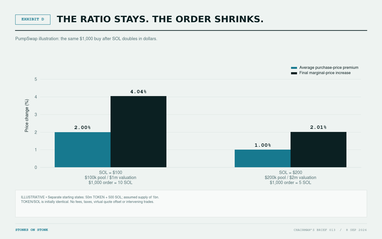
The ratio is unchanged, but $1,000 now buys half as many SOL. It is a smaller order against the same 500 SOL reserve.
A 10 SOL purchase still produces the original percentage impact. It simply costs $2,000.
Fixed-dollar orders and orders sized relative to market cap are different comparisons.
The table isolates curve effects. Fees change what the buyer receives. For this hypothetical canonical pool, the documented 10,000-SOL valuation tier is 0.20% LP, 0.05% protocol and 0.70% creator fees. With those explicit inputs, Pump’s SDK returns approximately 971,345 TOKEN for the $1,000 budget when SOL is $100. The average premium is 2.95%, and the ending marginal price increases 4.006%, including the LP fee retained in the pool. At SOL $200, the average premium is 1.95%. The SOL-denominated valuation remains 10,000 SOL, so the quote-only repricing does not change that tier. SOURCE 04Pump — FeesOpen source ↗SOURCE 17PumpSwap SDK 1.19.0Open source ↗
A separate sale of $1,000 of pre-trade marked inventory has an average discount of 2.892% at SOL $100, or 1.931% at SOL $200. These are hypothetical SDK calculations with zero virtual quote offset, not observations of a live Pump pool.
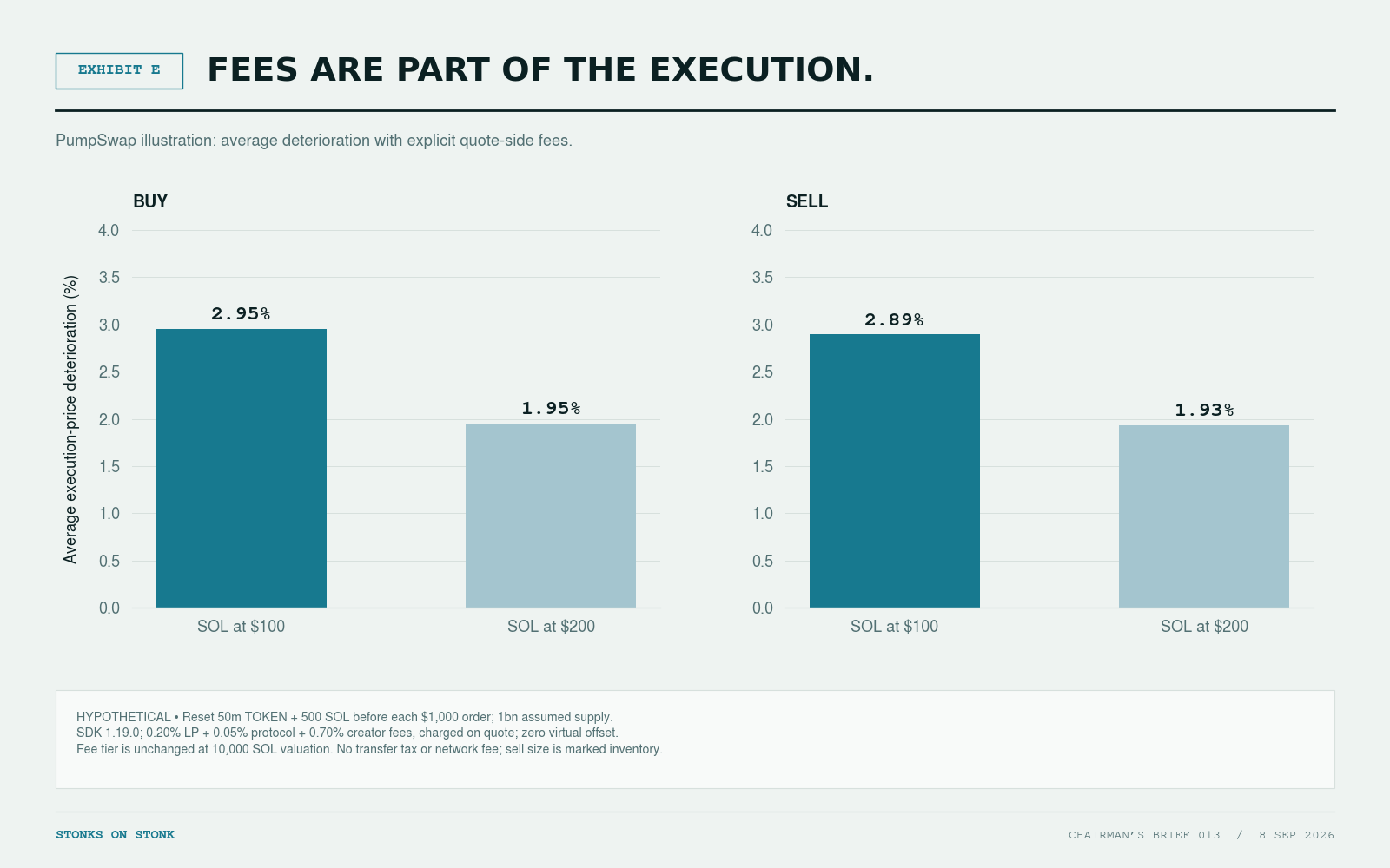
PumpSwap charges these fees on the quote amount: added to the curve’s quote requirement for a buy, deducted from quote output for a sell. Each component rounds up separately in the examined SDK. A generic “subtract the fee from every input” rule would misstate this example. SOURCE 17PumpSwap SDK 1.19.0Open source ↗
Before graduation, “reserves” means something else
Pump’s bonding curve separates virtual reserves used for pricing from real reserves tracking actual assets. Its program documentation describes buys increasing both quote-reserve measures by the corresponding net trade amount. Virtual reserves are not an equivalent quantity of withdrawable money. SOURCE 06Pump — Pump program READMEOpen source ↗
For a hypothetical point on such a curve, assume 50 SOL of virtual quote reserves, 20 SOL of real accumulated quote, SOL at $100, and enough sale tokens remaining to complete the next trade without graduating.
A fee-free $1,000 buy adds 10 SOL. Virtual quote reserves become 60 SOL; real quote reserves become 30 SOL.
The price calculation uses the virtual 50 SOL starting reserve. The calculated average purchase-price premium is 20%, and the final marginal-price increase is 44%.
Those figures describe an invented, fee-free curve state, not a typical Pump launch. Pump’s current published bonding-curve schedule totals 1.25%; an actual user budget must also cover the applicable fees. Neither the 50-SOL virtual reserve nor the 20-SOL real reserve is presented as a live launch parameter. SOURCE 04Pump — FeesOpen source ↗
The lesson is that the number governing price sensitivity need not equal the money actually collected. A pre-graduation liquidity display therefore cannot automatically be interpreted like a mature two-sided pool.
Pump’s documented completion condition is exhaustion of the real sale-token reserve. A SOL/USD rally alone does not exhaust those tokens merely by raising the displayed dollar valuation. SOURCE 06Pump — Pump program READMEOpen source ↗
Pump and StonkFun do not create every market the same way
A launch platform and an AMM are different layers. The relevant comparison is how each route creates inventory, then how its trading mechanism responds to orders.
| Route examined | Launch-stage trading | Subsequent market | What establishes liquidity? |
|---|---|---|---|
| Native Pump route | Virtual-reserve bonding curve | PumpSwap | Actual reserves delivered at migration |
| Legacy StonkFun direct-CLMM route | Real inventory offered through concentrated positions | Raydium CLMM | Token allocation, range boundaries and initial price |
| StonkFun LaunchLab route | Configured bonding curve | Raydium CPMM | Actual quote accumulated, remaining token allocation and migration deductions |
This is a comparison of relevant routes, not an exhaustive claim about every product mode, supported quote or pool either platform can create.
StonkFun’s direct-pool description specifies a one-sided Raydium market. In the legacy CLMM arrangement examined here, project inventory can be offered across price ranges; buying converts some of that inventory into quote assets. There is no separate curve-to-pool migration in a direct-CLMM launch. The exact positions of a particular token must be checked rather than inferred from the platform label. SOURCE 07StonkFun — Direct-pool launch descriptionOpen source ↗SOURCE 09Raydium — CLMM overviewOpen source ↗
StonkFun separately documents a LaunchLab constant-product route configured to migrate into CPMM, with quote selection and launch parameters supplied by its current configuration. That is not the same as saying every curve option available in LaunchLab is available through StonkFun. SOURCE 08StonkFun — Developer documentationOpen source ↗
LaunchLab keeps virtual pricing parameters, real quote accumulated and fee accounting distinct. The gross headline raise should not simply be equated with net quote entering the graduated pool. SOURCE 10Raydium — LaunchLab accountsOpen source ↗
The distinction is not “organized” versus “chaotic” price discovery. It is which inventory is available, under which pricing rule, at which stage.
Concentrated liquidity: the shelves have price labels
A full-range pool spreads liquidity over the constant-product curve. A concentrated-liquidity pool lets providers assign inventory to defined price ranges. Only positions covering the current relative price contribute active liquidity. SOURCE 09Raydium — CLMM overviewOpen source ↗
Think of the first as one continuous shelf and the second as shelves labelled with different prices. Total stock in the shop does not tell you how much is available on the shelf your order is about to reach.
A calculated example makes this concrete. Hold total pool value at $100,000, with the project and quote each priced at $1.
An ordinary full-range pool has 50,000 units on each side. A fee-free $1,000 buy produces the familiar 2% average premium and 4.04% marginal-price increase.
A hypothetical concentrated position also holds 50,000 units on each side, but covers 0.25 to 4 quote units per project token. Using concentrated-liquidity mathematics, the same buy produces a 1% average premium and 2.01% marginal-price increase, remaining inside its range. The appendix shows the calculation. SOURCE 11Raydium CLMM — pinned square-root-price mathematicsOpen source ↗
Same total value. Same starting inventory values. Different depth near spot.
The trade-off is that a position can become entirely one asset and cease supplying active liquidity when the relative price leaves its range. Other positions can remain active; crossing ranges can increase or decrease total active liquidity. It does not necessarily drain away in one direction. SOURCE 12Raydium — Ticks and positionsOpen source ↗
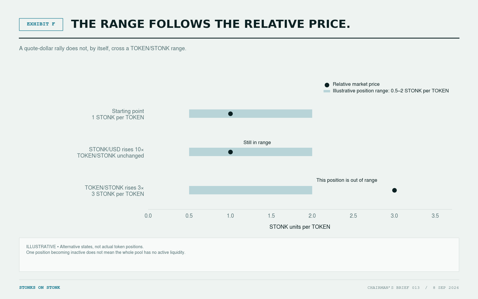
For a position covering 0.5 to 2 STONK per TOKEN, a 10× rise in STONK/USD changes nothing about range membership if TOKEN still trades for one STONK.
A move to three STONK per TOKEN is different: that particular position is outside its range.
The range follows the token-to-token price, not the dollar translation.
Open the pools: STONKS, DEX and KNOTS
This is why three STONK-quoted markets can show very different liquidity ratios without contradicting one another.
The account owners establish STONKS and DEX as Raydium CLMM, and KNOTS as Raydium CPMM. Each pool holds the specified project mint against the same STONK mint. DEX is tracked here by the mint previously labelled STONKDEX; a ticker rename does not create a different asset. SOURCE 13STONKS pool accountOpen source ↗SOURCE 14DEX pool accountOpen source ↗SOURCE 15KNOTS graduated pool accountOpen source ↗
The following accounts were read together at 11:04:32 UTC on 8 September 2026, finalized slot 445322492. STONK is marked at $0.15603773, using the contemporaneous STONK/USDC pool with the deepest active virtual USDC depth among the discovered CLMM markets and assuming one USDC equals one dollar. This is a valuation mark, not a quote for converting the whole position into dollars. SOURCE 18STONK/USDC valuation-reference poolOpen source ↗
| Common-slot measure | STONKS / STONK | DEX / STONK | KNOTS / STONK |
|---|---|---|---|
| AMM | CLMM | CLMM | CPMM |
| Project tokens in vault account | 492.262m | 319.927m | 45.708m |
| STONK in vault account | 1.262305m | 1.085777m | 1.112630m |
| Project-side marked value | $386.4k | $251.6k | $173.6k |
| STONK-side marked value | $197.0k | $169.4k | $173.6k |
| Combined vault value | $583.4k | $421.0k | $347.2k |
| Current mint supply | 991.781m | 966.443m | 999.457m |
| Price × current mint supply | $778.5k | $760.0k | $3,796.4k |
| Vault value / that valuation | 74.9% | 55.4% | 9.1% |
Calculated from raw accounts in the evidence bundle. “Current mint supply” is explicit: it is not certified circulating supply, and it is not the one-billion-token initial-supply convention. Vault amounts include separately accounted pool fees but exclude the Token-2022 account’s separately withheld transfer-fee balance. Amounts and dollars are rounded here; raw integers are retained.
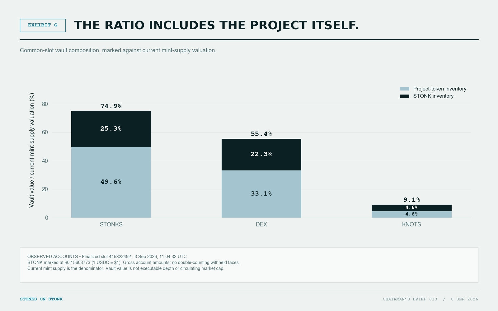
STONKS: a large inventory of its own token
Approximately two-thirds of the vault’s marked value is STONKS itself. The 74.9% ratio does not mean 74.9% of valuation is held as STONK ready to pay sellers.
The initial position transaction, on 5 August at 22:57:00 UTC, deposited roughly 150 million and 850 million STONKS, both into the same tick interval, −54840 to 67080, with no STONK deposited. The pool had been created two seconds earlier; the first successful swap found in the launch window followed at 22:57:02. These are distinct events. SOURCE 19STONKS initial position transactionOpen source ↗
Today, the original broad interval’s aggregate liquidity is still present in net terms, alongside three smaller intervals. Only two intervals cover the current price; two smaller intervals are out of range. That describes the present distribution, not proof that no intervening deposits or withdrawals occurred.
STONKS uses the legacy SPL Token program and has no Token-2022 transfer fee. Its examined CLMM configuration instead charges 4% on STONK: the input on a buy and the output on a sell. Calling this a 4% tax on every STONKS transfer would describe the wrong mechanism. SOURCE 13STONKS pool accountOpen source ↗SOURCE 20Raydium CLMM — pinned swap mathematicsOpen source ↗
DEX: the same AMM family, not the same pool
DEX’s STONK inventory is about 14% smaller than STONKS’s, while its headline ratio is much lower. The two questions require different denominators.
On 14 August at 22:55:28 UTC, DEX’s launch transaction opened two positions with approximately 900 million and 100 million tokens sent. A 3% transfer fee left approximately 873 million and 97 million in the pool. Both positions used ticks −46920 to 75000. The same transaction included a first buy. SOURCE 21DEX initial position and buy transactionOpen source ↗
The original DEX and STONKS ranges span the same number of ticks, but their absolute starting prices, deposit splits, net inventory and fee structures differ. That is useful comparative evidence. It is not a controlled experiment in launch timing.
DEX currently has one aggregate active interval. Its 1% CLMM fee is charged on STONK, while the 3% Token-2022 transfer fee applies to DEX. On a buy, quote-side fees reduce the amount driving the curve, then the output transfer reduces tokens delivered. On a sell, the input transfer reduces tokens reaching the pool, then the quote-side pool fee reduces STONK delivered. Adding the percentages together is only a rough shorthand. SOURCE 14DEX pool accountOpen source ↗SOURCE 20Raydium CLMM — pinned swap mathematicsOpen source ↗
KNOTS: similar-order quote inventory, a different valuation and curve
KNOTS holds about 1.113 million STONK, close to DEX’s 1.086 million, against a much larger current-mint-supply valuation. Its effective CPMM reserves have equal marked value by the reserve-price identity; the two gross account values differ slightly because fee balances are included.
Here the launch provenance is directly recoverable. KNOTS initialized a Token-2022 LaunchLab curve on 5 September at 16:34:16 UTC, with a buy in that transaction. It migrated to the identified CPMM on 6 September at 05:58:04 UTC. The original curve account and the graduated pool are different accounts. SOURCE 22KNOTS initializationOpen source ↗
The stored fundraising target was 222,844.764611314 STONK. The migration transaction recorded 222,844.764611753 STONK entering the CPMM and 200.693 million net KNOTS. The remaining gross allocation was 206.9 million KNOTS; its 3% transfer fee accounts for the 6.207-million-token difference. The transaction also locked LP tokens. These are this launch’s observed amounts, not universal graduation constants. SOURCE 22KNOTS initializationOpen source ↗
Later liquidity additions are visible. Two verified deposits shortly before the snapshot added about 1,145.677 and 14,985.127 STONK, together with the corresponding net KNOTS. The LP supply and reserve product also grew between migration and the snapshot. The original invariant cannot simply be carried forward unchanged. The bundle records these additions without claiming a complete deposit-and-withdrawal history. SOURCE 23KNOTS later liquidity additionOpen source ↗
KNOTS combines a 0.25% input-side trading fee, a 1% creator fee charged on STONK, and a 3% KNOTS transfer fee. Its effective reserves exclude accrued protocol, fund and creator fees; LP fees retained in the pool remain part of reserves. SOURCE 15KNOTS graduated pool accountOpen source ↗SOURCE 24Raydium CPMM — pinned curve calculatorOpen source ↗
STONKS versus DEX asks what differs within concentrated liquidity. KNOTS adds a different liquidity architecture. None of the three ratios, on its own, ranks the next trade’s execution.
The reconstructed orders make the distinction measurable. Each order below starts independently from the same snapshot; STONK/USD remains fixed. Buys spend $1,000 of STONK. Sells send tokens worth $1,000 at the starting marginal price, so their proceeds are lower than $1,000.
| $1,000 marked order | STONKS | DEX | KNOTS |
|---|---|---|---|
| Buy: average price premium | 4.424% | 4.541% | 4.992% |
| Buy: terminal marginal-price increase | 0.496% | 0.783% | 1.142% |
| Sell: average price discount | 4.247% | 4.336% | 4.741% |
| Sell: terminal marginal-price decline | 0.514% | 0.761% | 1.107% |
Reconstructed quotes include the identified fees, transfer taxes, tick traversal and integer rounding. Terminal movement measures the resulting pool price; average execution compares what the trader pays and receives with pre-trade spot. These are internal research calculations, not signed transaction simulations or an independently approved execution service.
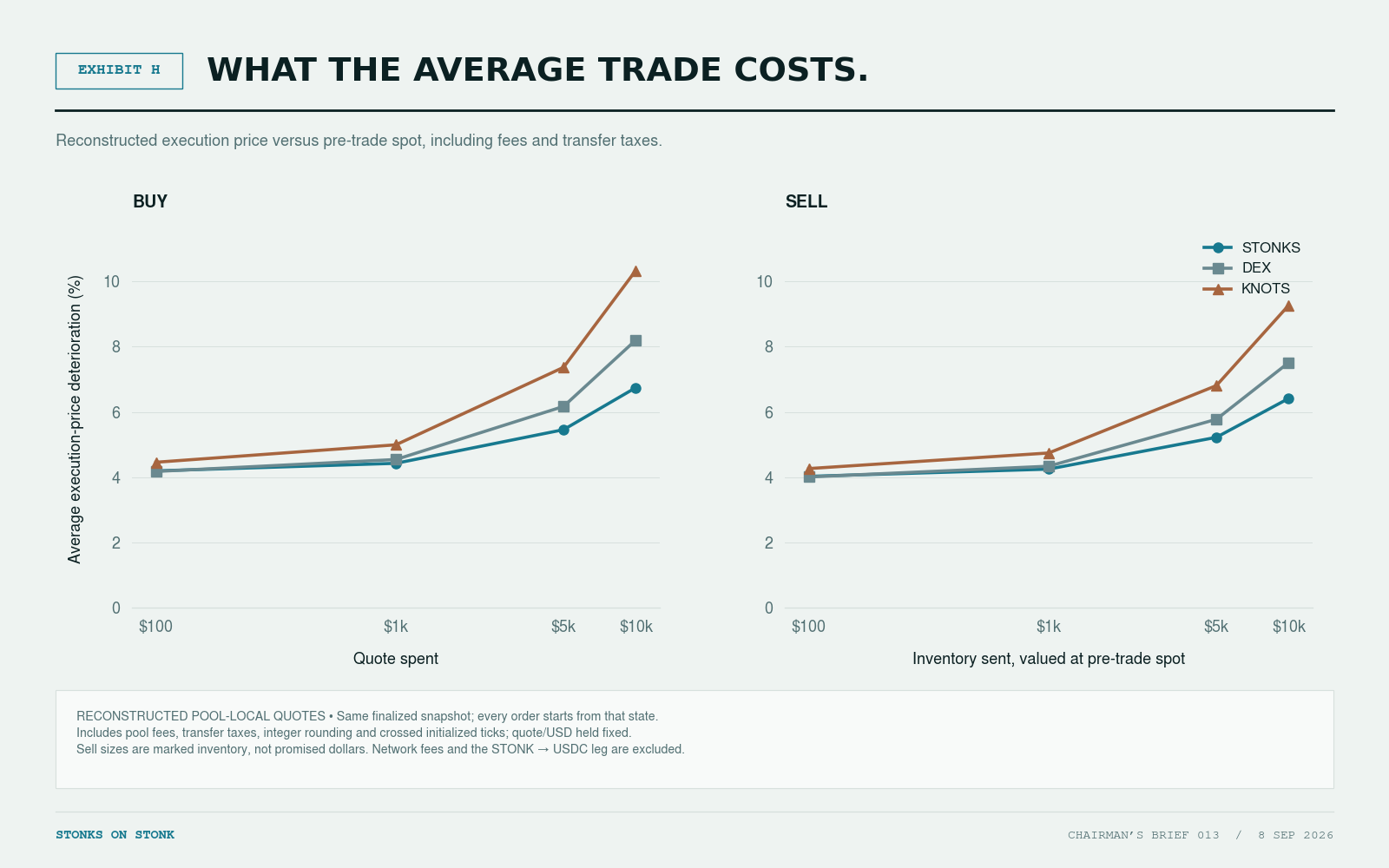
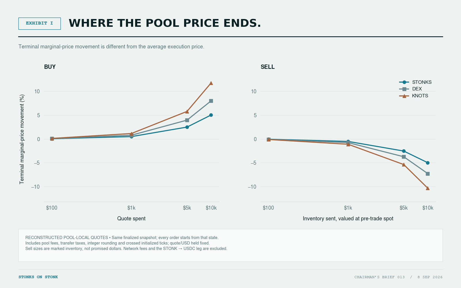
A substantial average execution cost can coexist with a small candle because fees and transfer taxes do not all move the curve. Conversely, a terminal price move describes the final marginal quote, not the average price of the trade.
Sizing orders as percentages of valuation changes the experiment again. Five percent is approximately $38.9k in STONKS, $38.0k in DEX and $189.8k in KNOTS. The STONKS buy crosses an initialized boundary and adds active liquidity; the sell crosses a different boundary and removes a small active interval. Those changes are included in the calculations.
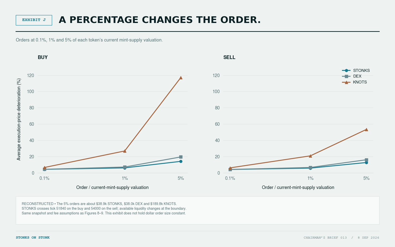
The complete 42-row table includes amounts sent and received, individual fee amounts, average execution, output shortfall, terminal movement and crossed ticks. All results stop at the TOKEN/STONK pool. An onward STONK-to-USDC trade requires another calculation.
Where launch timing actually enters
Consider two fictional tokens, each opening at a $1 token price with the same supply.
Token A launches when STONK is $1. Its initial exchange rate is one STONK per token.
Token B launches later, when STONK is $10. Its initial exchange rate is 0.1 STONK per token.
If A remains unchanged against STONK during that appreciation, it is worth $10 when B opens at $1.
They began at the same dollar price. They did not begin at the same relative price or experience the same denominator move.
That does not automatically give A a better liquidity ratio. Its unchanged inventory would also have appreciated in dollars.
Timing can also matter between launch and graduation. StonkFun specifies its LaunchLab fundraising input in quote-token units, sized from a pricing response at request time. SOURCE 08StonkFun — Developer documentationOpen source ↗
For a hypothetical launch with a fixed stored requirement of 100,000 STONK, those units represent $10,000 at $0.10 per STONK and $30,000 at $0.30. The quantity is unchanged; its dollar value is not. KNOTS’ separately verified target was approximately 222,844.765 STONK; the hypothetical number is retained to make the arithmetic readable.
A quote rally does not itself add quote units to the curve. It changes the dollar value represented by the existing units and target. The net quote delivered at graduation must still account for the applicable deductions. SOURCE 10Raydium — LaunchLab accountsOpen source ↗
A calendar date is not an AMM parameter. The prices, settings and trading history attached to that date are what matter.
In the idealized fee-free constant-product model, identical initial reserves and an identical ending relative price produce identical ending reserves. Real histories can differ because fees, liquidity decisions, configuration changes and participants differ—not because the calendar independently changes the equation.
The available launch records establish different starting conditions, and the common snapshot establishes today’s state. They do not establish a complete aligned TOKEN/STONK and STONK/USD return history. The bundle records the elapsed-time observations that could be recovered and marks unavailable windows explicitly; it does not interpolate missing price evidence. KNOTS has not yet reached +7 or +30 days after graduation, and DEX has not reached +30 days after its first trade.
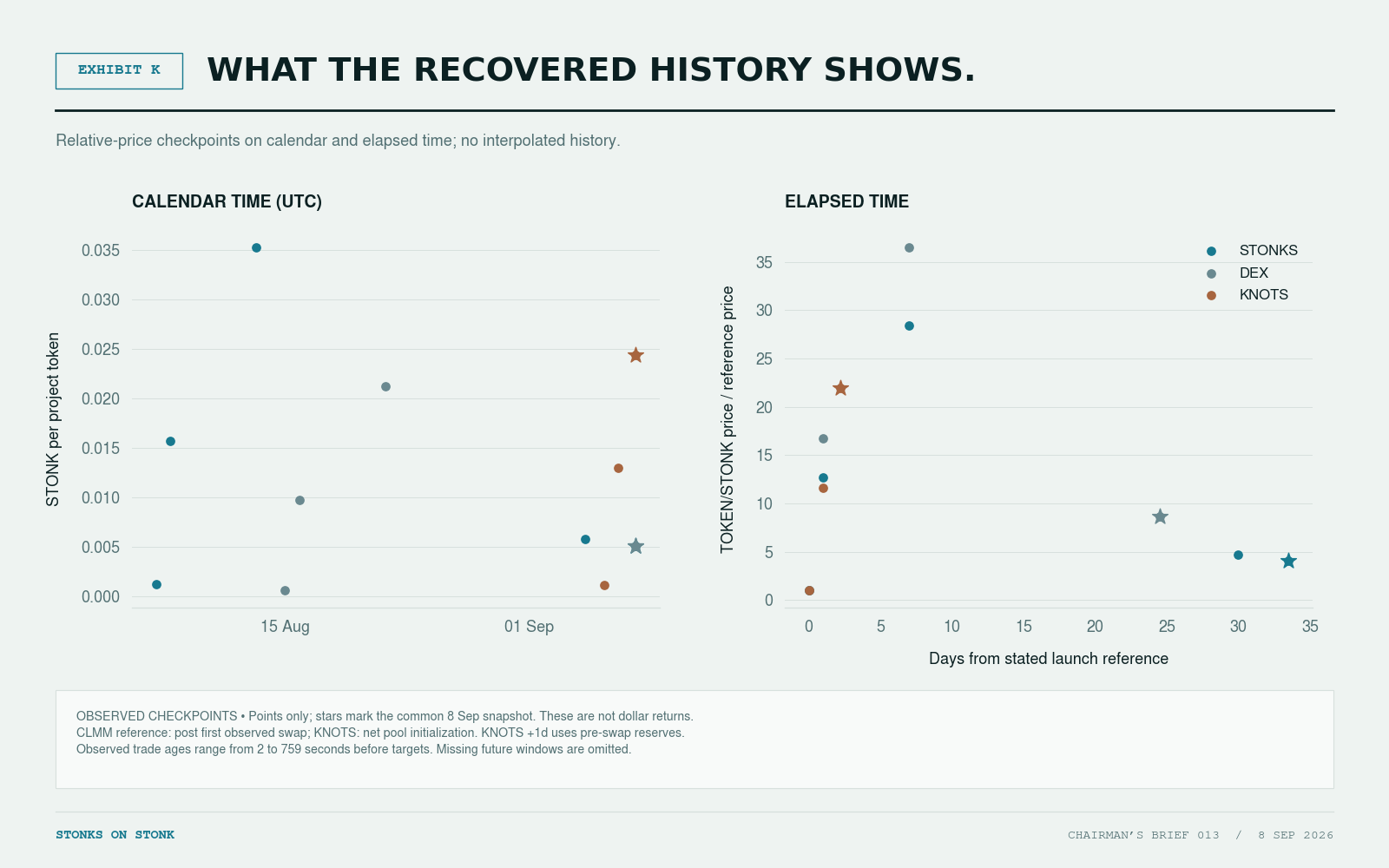
For observed price endpoints, the identity remains TOKEN/USD return factor = TOKEN/STONK return factor × STONK/USD return factor. Without aligned quote-price observations, a dollar return cannot honestly be apportioned between those factors. Rewards, transfers, burns and holder cash flows require separate total-return accounting.
Translation is not yet reflexivity
Quote translation is arithmetic. Reflexivity requires something to respond.
One possible feedback sequence is that STONK appreciates, a paired token’s dollar chart rises, the chart attracts attention, and new buyers then bid the token up against STONK itself. A 10× quote move combined with a 3× relative move becomes a 30× dollar move.
But that is a hypothesis about behaviour, not a built-in promise. A quote rally could instead prompt holders to sell the project for more STONK. The relative-price decline could offset part or all of the dollar benefit.
A thin interval of liquidity can amplify a particular order. It does not mechanically create buyers or determine the direction of the next order. Nor is denomination exposure the same thing as contractual leverage.
For the three case studies, proving a feedback effect requires trading and price evidence beyond a correlation between their dollar charts.
The useful comparison is not a podium
The correct conclusion is not that Pump wins, StonkFun wins, CPMM wins or CLMM wins.
Concentration can improve execution near a particular price while introducing range dependence. Full-range liquidity avoids chosen position boundaries but still produces price impact. A curve creates a different path into a mature pool from a direct liquidity launch. A volatile quote adds another moving price to the dollar result. SOURCE 03Pump — Bonding-curve overviewOpen source ↗SOURCE 09Raydium — CLMM overviewOpen source ↗SOURCE 10Raydium — LaunchLab accountsOpen source ↗
A market can look large while being difficult to trade. A pool can look large because it contains considerable project inventory. A dollar chart can rise because its denominator rose.
The questions are therefore connected: what is the token priced in, what inventory is actually held, where is it available, and what would a trade of this size do to it?
Selling into STONK is also not the same as exiting into dollars. Converting onward into another asset adds a separate market and its own execution conditions.
Before comparing the charts, compare the markets producing them.
Management has not ranked the plumbing.
Management would simply prefer that everyone knows which pipes they are standing on.
Chairman Stonks
Chairman & Chief Number Officer
Stonks on Stonk
Technical appendix: the arithmetic behind the examples
Valuation and supply
Use x for project-token inventory, y for quote inventory, p for quote units per project token, q for dollars per quote unit, and S for the chosen supply measure. Mark both reserves consistently at the same marginal prices:
Pool value V = q(xp + y)
Market value M = Spq
V / M = (x + y/p) / S
The quote-dollar price cancels. This valuation identity does not assert that every asset can be sold at the marginal price. It also does not turn gross vault balances into executable reserves.
Use circulating supply when claiming circulating market cap, and the appropriate total/diluted supply when claiming FDV. Here the teaching examples explicitly assume a fixed supply; the observed table uses the on-chain mint supply at the common snapshot. Mint supply can include restricted or otherwise non-circulating holdings, so this denominator is labelled rather than called circulating market cap.
Fee-free real-reserve constant product
With xy = k and p = y/x, the ratio simplifies to V/M = 2x/S.
If the relative-price multiple is r and the quote-dollar multiple is Q:
x₁ = x₀ / √r
y₁ = y₀ √r
V₁/V₀ = Q√r
M₁/M₀ = Qr
(V/M)₁ / (V/M)₀ = 1/√r
A buy adds b quote units and receives a = xb/(y+b) project units. Its average purchase-price premium over the starting price is b/y; its terminal marginal-price increase is (1+b/y)² − 1. These are deliberately different measures. Relative to a no-impact output quote, the output shortfall is b/(y+b), not b/y.
For a sell of a project units, the quote received is ya/(x+a). The average sale-price discount is a/(x+a) and the terminal marginal-price decline is 1 − (1+a/x)⁻². This explains why exact buy and sell percentages are not symmetric.
With dollar buy size B and pre-trade pool value V, holding quote/USD fixed, b/y = 2B/V. If B is a fraction f of market value and the liquidity ratio is ℓ, then b/y = 2f/ℓ.
Concentrated-liquidity calculation
Normalize price as quote units per project token. For a position with lower bound pₐ, upper bound pᵦ and p inside the range:
x = L(1/√p − 1/√pᵦ)
y = L(√p − √pₐ)
In the worked example, p = 1, pₐ = 0.25, pᵦ = 4, and L = 100,000, giving x = y = 50,000. A 1,000-unit quote buy changes √p to 1 + 1,000/100,000 = 1.01. It receives about 990.099 project tokens: a 1% average premium and a 2.01% terminal price increase. The price remains inside the position’s range. SOURCE 11Raydium CLMM — pinned square-root-price mathematicsOpen source ↗
This is an idealized continuous-price example, not a Raydium integer-accurate execution quote. Actual calculations require token ordering and decimals, permitted ticks, all crossed ranges, fees and rounding.
Observed execution and reserve reconciliation
The observed pools put STONK in token0 and the project token in token1. Raydium’s stored square-root price represents raw token1/token0. The article’s STONK-per-project price therefore inverts its square and adjusts for decimals. A STONK-input buy decreases the stored square-root price; a project-input sell increases it. Some prose documentation reverses this direction; the calculations follow source code and emitted transaction events.
For CLMM, the script reconstructs piecewise principal from all initialized liquidity intervals, using integer Q64.64 arithmetic. It verifies that net liquidity across all boundaries sums to zero and that liquidity below the current tick equals the pool’s active liquidity. Dynamic-fee fields and limit-order quantities are zero in both examined case-study pools. Gross balances minus reconstructed principal and separately accounted protocol/fund fees leave small residuals; these are reported as accrued-fee/dust residuals, not falsely assigned to individual LP positions.
For KNOTS, effective quote reserves are 1,112,278.704731742 STONK and effective project reserves are 45,691,582.500741 KNOTS. Both subtract separately accounted fees from token-account amounts. Withheld transfer taxes live outside those amounts and are not subtracted a second time.
Buy average deterioration is paid quote / received project / initial price − 1. Sell average deterioration is 1 − received quote / sent project / initial price. Output shortfall instead compares received output with the no-impact output implied by the gross input. Terminal movement is ending marginal price / starting marginal price − 1; sells therefore have a negative terminal movement in the data table.
Protocol and evidence boundaries
PumpSwap quoting must use effective quote reserves, including any configured virtual adjustment. The PumpSwap illustration sets that adjustment to zero. SOURCE 05Pump — PumpSwap program READMEOpen source ↗
Raydium CPMM effective trading reserves exclude separately accounted fees; raw vault balances alone can overstate tradable reserves. Transfer-fee tokens can reduce input received or output delivered. CLMM requires position/tick-aware calculations, not p = y/x on aggregate balances. SOURCE 11Raydium CLMM — pinned square-root-price mathematicsOpen source ↗SOURCE 16Raydium CPMM — pool accountingOpen source ↗
Teaching Exhibits A–D and F exclude fees and taxes. Exhibit E supplies explicit Pump fees. Observed Exhibits G–J use the account and fee state described above. All trade comparisons exclude network fees, external trades and simultaneous liquidity changes. They show pool-local outcomes, not guaranteed routed execution or future prices. Holder distributions are outside these price-only examples; price appreciation is not a rewards-adjusted total return.
The bundle contains raw account responses, launch and migration transactions, source pins, reusable calculation scripts and internal checks, including replay of consecutive historical CLMM swaps and comparison with the Raydium SDK. Program IDs and deployment slots are recorded. A reproducible build matching the deployed binaries, full historical cash-flow reconciliation and independent technical approval remain outstanding. The calculations are internally checked research, not independently approved execution quotes. Missing history is not replaced with estimates.
Sources and reading notes
Sources checked on 8 September 2026. Raw Solana RPC records and calculation outputs are included in the evidence bundle. Explorer links identify the same accounts or transactions; the numerical snapshot comes from the saved RPC response, not a later explorer display. Download the frozen evidence and calculation bundle.
- Uniswap — V2 pricing. Reserve-based price formation and swap accounting.
- Raydium — Slippage and price impact. Used for the conceptual distinction between quoted impact and execution slippage; numerical examples are independently derived.
- Pump — Bonding-curve overview. Native curve-to-PumpSwap pathway.
- Pump — Fees. Current SOL/USDC quote options and fee schedule; the additional SDK illustration states its fee inputs explicitly.
- Pump — PumpSwap program README. Constant-product baseline and effective quote reserves. Read blob:
19192cf7e3d4f7c07be0c32959dbd94aedd9430c. - Pump — Pump program README. Virtual/real reserves and completion condition. Read blob:
27f4eb82aea8e34db6c2b997837b3e9f282ebfe1. - StonkFun — Direct-pool launch description. One-sided market description; not proof of the current availability or initial settings of every route.
- StonkFun — Developer documentation. LaunchLab path, supported configuration and quote-unit fundraising sizing.
- Raydium — CLMM overview. Concentrated liquidity and active ranges.
- Raydium — LaunchLab accounts. Real/virtual amounts, quote-unit target and fee/migration accounting.
- Raydium CLMM — pinned square-root-price mathematics. Token ordering and integer rounding; source code takes precedence over inconsistent prose direction labels.
- Raydium — Ticks and positions. Range boundaries and changes in active liquidity.
- STONKS pool account. Pool, vaults, mint and fee configuration are in the saved common-slot RPC response.
- DEX pool account. Same snapshot and linked Token-2022 mint configuration.
- KNOTS graduated pool account. Same snapshot and linked CPMM fee configuration.
- Raydium CPMM — pool accounting. Exclusion of separately accounted fees.
- PumpSwap SDK 1.19.0. Buy/sell math, separate quote-side fee ceilings and virtual reserve adjustment. Pinned in the included package lock.
- STONK/USDC valuation-reference pool. Same-slot raw square-root price; selection and alternative marks in
data/quote_mark.json. - STONKS initial position transaction. Original net deposits, ranges and emitted liquidity; first-swap evidence is separate in the bundle.
- Raydium CLMM — pinned swap mathematics. Input/output fee placement and integer arithmetic. Token transfer fees are read from each mint.
- DEX initial position and buy transaction. Deposits, transfer deductions, range and first buy.
- KNOTS initialization and migration. LaunchLab account, target, net migrated reserves and LP locking.
- KNOTS later liquidity addition and second verified addition. Emitted net reserve additions and transfer fees.
- Raydium CPMM — pinned curve calculator. Trading/creator fee split, output calculation and rounding.
Teaching examples are hypothetical. Observed comparisons are reconstructed, pool-local outcomes at the stated snapshot, not guaranteed routed execution or future prices. Internal calculation checks are not independent technical approval.
Return to the Chairman's Office →